Getting started
Run this example in colab!
In this example, we use the BayHess package to assist MICE in minimizing a quadratic function. Let the quadratic function \(f\) to minimized be
where
Here, we have a Hessian that is a convex combination of the identity matrix and of an arbitrary matrix:
noting that \(\theta\) is a random variable such that \(\theta \sim \mathcal{U}[0, 1]\) and \(\kappa\) is the desired conditioning number of the expected value of the Hessian. Also, \(\boldsymbol{b}\) is a 2-dimensional vector with ones.
To use the stochastic gradient method, we need the gradient of \(f\) wrt \(\boldsymbol{\xi}\):
First, let’s install both MICE and BayHess from PyPI using pip.
%pip install -U mice
%pip install -U bayhess
Requirement already satisfied: mice in /home/andre/miniconda3/envs/p39/lib/python3.9/site-packages (0.1.27)
Requirement already satisfied: matplotlib>=3.2.0 in /home/andre/miniconda3/envs/p39/lib/python3.9/site-packages (from mice) (3.4.2)
Requirement already satisfied: pandas>=1.1 in /home/andre/miniconda3/envs/p39/lib/python3.9/site-packages (from mice) (1.3.2)
Requirement already satisfied: numpy>=1.19 in /home/andre/miniconda3/envs/p39/lib/python3.9/site-packages (from mice) (1.20.3)
Requirement already satisfied: scipy>=1.8.1 in /home/andre/miniconda3/envs/p39/lib/python3.9/site-packages (from mice) (1.8.1)
Requirement already satisfied: pillow>=6.2.0 in /home/andre/miniconda3/envs/p39/lib/python3.9/site-packages (from matplotlib>=3.2.0->mice) (9.2.0)
Requirement already satisfied: python-dateutil>=2.7 in /home/andre/miniconda3/envs/p39/lib/python3.9/site-packages (from matplotlib>=3.2.0->mice) (2.8.2)
Requirement already satisfied: cycler>=0.10 in /home/andre/miniconda3/envs/p39/lib/python3.9/site-packages (from matplotlib>=3.2.0->mice) (0.11.0)
Requirement already satisfied: pyparsing>=2.2.1 in /home/andre/miniconda3/envs/p39/lib/python3.9/site-packages (from matplotlib>=3.2.0->mice) (3.0.4)
Requirement already satisfied: kiwisolver>=1.0.1 in /home/andre/miniconda3/envs/p39/lib/python3.9/site-packages (from matplotlib>=3.2.0->mice) (1.4.2)
Requirement already satisfied: pytz>=2017.3 in /home/andre/miniconda3/envs/p39/lib/python3.9/site-packages (from pandas>=1.1->mice) (2022.1)
Requirement already satisfied: six>=1.5 in /home/andre/miniconda3/envs/p39/lib/python3.9/site-packages (from python-dateutil>=2.7->matplotlib>=3.2.0->mice) (1.16.0)
Note: you may need to restart the kernel to use updated packages.
Requirement already satisfied: bayhess in /home/andre/miniconda3/envs/p39/lib/python3.9/site-packages (0.1.2)
Requirement already satisfied: numpy>=1.19 in /home/andre/miniconda3/envs/p39/lib/python3.9/site-packages (from bayhess) (1.20.3)
Requirement already satisfied: scipy>=1.7.1 in /home/andre/miniconda3/envs/p39/lib/python3.9/site-packages (from bayhess) (1.8.1)
Note: you may need to restart the kernel to use updated packages.
To use MICE to estimate \(\nabla_{\boldsymbol{\xi}} f\), we need to import the MICE class and NumPy to assist us in defining our problem. We also import the BayHess class to be used soon.
import matplotlib.pyplot as plt
import numpy as np
from numpy.linalg import solve, norm
from mice import MICE, plot_mice
from bayhess import BayHess
Then, we need to define \(\nabla_{\boldsymbol{\xi}} f\) as a function of \(\boldsymbol{\xi}\) and an array representing a sample of \(\theta\).
kappa = 100
H_aux = np.array([[kappa, kappa-1], [kappa-1, kappa]])
true_hess = np.array([[kappa+1, kappa-1], [kappa-1, kappa+1]])/2
b = np.ones(2)


def dobjf(x, thetas):
    gradients = []
    for theta in thetas:
        H = np.eye(2) * (1 - theta) + H_aux * theta
        gradients.append(H @ x.T - b)
    return np.vstack(gradients)
As for \(\theta\), we can pass to MICE either a sampler function that takes the desired sample size as input and returns the sample or a list/array containing the data. Here, we will define a function that returns the uniform sample between 0 and 1,
def sampler(n):
    return np.random.uniform(0, 1, int(n))
Now, let’s create an instance of MICE to solve this optimization problem with tolerance to statistical error of \(\epsilon=0.7\), maximum cost of \(10,000\) evaluations of \(\nabla_{\boldsymbol{\xi}} f\), and a minimum batch size of \(5\).
df = MICE(dobjf,
          sampler=sampler,
          eps=.7,
          min_batch=5,
          stop_crit_norm=0.1)
To perform optimization, we need to set a starting point and a step size. Here, we know both the \(L\)-smoothness and the \(\mu\)-convexity parameters of the problem, thus we can set the step size optimally.
x = np.array([20., 50.])
L = kappa
mu = 1
step_size = 2 / (L + mu) / (1 + df.eps ** 2)
and, finally, we iterate until MICE’s cost is reached, in which case df.terminate returns True,
while True:
    grad = df(x)
    if df.terminate:
        break
    x = x - step_size * grad
The method get_log returns a Pandas DataFrame with the information of what happened each iteration
log = df.get_log()
log
| event | num_grads | vl | bias_rel_err | grad_norm | iteration | hier_length | |
|---|---|---|---|---|---|---|---|
| 0 | start | 50 | 6.588308e+06 | 0.000000 | 4695.389187 | 1 | 1 |
| 1 | MICE | 326 | 1.375789e+07 | 0.102251 | 1227.318777 | 2 | 2 |
| 2 | dropped | 494 | 6.215808e+05 | 0.323431 | 967.609250 | 3 | 3 |
| 3 | restart | 564 | 3.010972e+05 | 0.000000 | 876.481800 | 4 | 1 |
| 4 | dropped | 584 | 3.173592e+05 | 0.135645 | 545.465263 | 5 | 2 |
| ... | ... | ... | ... | ... | ... | ... | ... |
| 404 | dropped | 12330 | 1.101072e-04 | 0.663222 | 0.095459 | 405 | 10 |
| 405 | dropped | 12370 | 2.859101e-05 | 0.645569 | 0.094172 | 406 | 10 |
| 406 | dropped | 12400 | 6.243965e-05 | 0.650190 | 0.094283 | 407 | 10 |
| 407 | dropped | 12440 | 4.125492e-05 | 0.650354 | 0.091576 | 408 | 10 |
| 408 | end | 12480 | 4.103791e-05 | 0.648924 | 0.090381 | 409 | 10 |
409 rows × 7 columns
Now, let’s plot the convergence of the norm of MICE’s gradient estimates from the log DataFrame using the built-in plot_mice function.
fig, ax = plt.subplots(figsize=(6, 5))
ax = plot_mice(log, ax, 'iteration', 'grad_norm', style='semilogy')
ax.axhline(df.stop_crit_norm, ls='--', c='k', label='Gradient norm tolerance')
ax.set_xlabel('Iteration')
ax.set_ylabel('Norm of estimate')
ax.legend()
<matplotlib.legend.Legend at 0x7fd955869fa0>
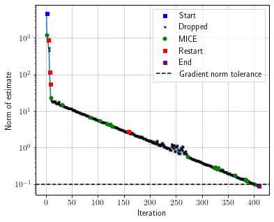
Note that SGD-MICE required 411 iterations to reach the gradient norm tolerance. Let’s use BayHess to obtain a Hessian approximation and pre-condition the gradient with its inverse. Before, we will create another instance of MICE.
df_ = MICE(dobjf,
          sampler=sampler,
          eps=.7,
          min_batch=5,
          stop_crit_norm=0.1)
And now, an instance of BayHess with \(\beta=10^{-2}\) and \(\rho=10^{-2}\).
bay = BayHess(n_dim=2, strong_conv=1, smooth=kappa,
              penal=1e-2, reg_param=1e-2)
Setting the same startin point as for SGD-MICE and a corresponding step size of \(1/(1 + \epsilon^2)\),
x = np.array([20., 50.])
step_size = 1 / (1 + df.eps ** 2)
we can perform optimization using SGD-MICE-Bay.
while True:
    grad = df_.evaluate(x)
    bay.update_curv_pairs_mice(df_)
    if not df_.k % 3:
        bay.find_hess()
    if df_.terminate:
        break
    x = x - step_size * solve(bay.hess, grad)
Similarly to what we have done before, we can check MICE’s log
log_ = df_.get_log()
log_
| event | num_grads | vl | bias_rel_err | grad_norm | iteration | hier_length | |
|---|---|---|---|---|---|---|---|
| 0 | start | 50 | 8.206547e+06 | 0.000000 | 4358.977188 | 1 | 1 |
| 1 | restart | 110 | 2.305343e+05 | 0.000000 | 913.121963 | 2 | 1 |
| 2 | dropped | 200 | 4.531934e+05 | 0.228281 | 283.607233 | 3 | 2 |
| 3 | restart | 270 | 9.738793e+03 | 0.000000 | 173.316025 | 4 | 1 |
| 4 | dropped | 302 | 5.558856e+03 | 0.248118 | 53.630654 | 5 | 2 |
| 5 | restart | 372 | 2.414530e+02 | 0.000000 | 30.321476 | 6 | 1 |
| 6 | dropped | 382 | 7.639652e+01 | 0.122466 | 17.108728 | 7 | 2 |
| 7 | dropped | 402 | 1.583018e+02 | 0.160855 | 13.025718 | 8 | 2 |
| 8 | dropped | 442 | 2.286118e+02 | 0.257132 | 8.148506 | 9 | 2 |
| 9 | restart | 512 | 6.888974e+00 | 0.000000 | 4.512811 | 10 | 1 |
| 10 | dropped | 532 | 2.132636e+00 | 0.261287 | 1.354497 | 11 | 2 |
| 11 | restart | 602 | 1.113125e+00 | 0.000000 | 0.679711 | 12 | 1 |
| 12 | dropped | 672 | 2.213795e-02 | 0.257727 | 0.281719 | 13 | 2 |
| 13 | end | 1113 | 6.260119e-01 | 0.000000 | 0.058472 | 14 | 1 |
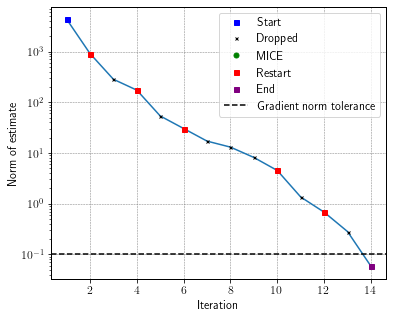
And make a convergence plot.
fig, ax = plt.subplots(figsize=(6, 5))
ax = plot_mice(log_, ax, 'iteration', 'grad_norm', style='semilogy')
ax.axhline(df_.stop_crit_norm, ls='--', c='k', label='Gradient norm tolerance')
ax.set_xlabel('Iteration')
ax.set_ylabel('Norm of estimate')
ax.legend()
<matplotlib.legend.Legend at 0x7fd9557a0f70>
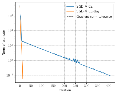
To better illustrate the difference, let’s make a convergence plot comparing SGD-MICE with and without the Bayesian Hessian pre-conditioning.
fig, ax = plt.subplots(figsize=(6, 5))
ax.semilogy(log["grad_norm"], label="SGD-MICE")
ax.semilogy(log_["grad_norm"], label="SGD-MICE-Bay")
ax.axhline(df_.stop_crit_norm, ls='--', c='k', label='Gradient norm tolerance')
ax.set_xlabel('Iteration')
ax.set_ylabel('Norm of estimate')
ax.legend()
<matplotlib.legend.Legend at 0x7fd9555f5f70>
Still, due to MICE’s adaptive control of the relative statistical error, the number of gradient evaluations changes per iteration. Let’s take a look at the convergence versus the number of gradient evaluations.
fig, ax = plt.subplots(figsize=(6, 5))
ax.loglog(log["num_grads"], log["grad_norm"], label="SGD-MICE")
ax.loglog(log_["num_grads"], log_["grad_norm"], label="SGD-MICE-Bay")
ax.axhline(df_.stop_crit_norm, ls='--', c='k', label='Gradient norm tolerance')
ax.set_xlabel('Gradient evaluations')
ax.set_ylabel('Norm of estimate')
ax.legend()
<matplotlib.legend.Legend at 0x7fd955af0610>
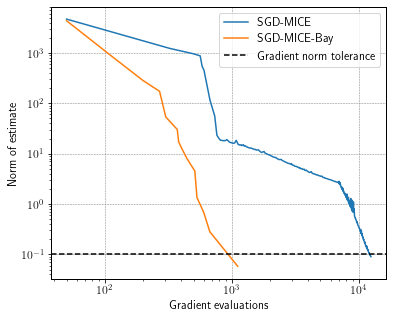
Using the Hessian approximation from BayHess resulted in a dramatic reduction in the cost of achieving the desired tolerance.
reduction = (log["num_grads"].max() - log_["num_grads"].max()) / log["num_grads"].max()*100
print(f"BayHess reduced the overall cost in {reduction:.3f} %")
BayHess reduced the overall cost in 91.082 %